Code Completion Using Machine Learning
An overview of modern methods
Aaron Davis
Data Science
University of Colorado
Boulder, CO, USA
[email protected]
Darsh Shah
Data Science
University of Colorado
Boulder, CO, USA
[email protected]
Faizan Husain
Data Science
University of Colorado
Boulder, CO, USA
[email protected]
Spriha Awasthi
Data Science
University of Colorado
Boulder, CO, USA
[email protected]
Abstract
During this project, we focus on creating better code autocompletion for Python IDEs using machine learning. The specific methods we use are n-gram code completion, RNN and LSTM code completion, and Transformer networks for code completion. The primary result of this project is an LSTM network that achieved 86% accuracy on a validation dataset. The conclusion of this project is that using machine learning for code completion is a fairly difficult task, but the results justify the time and effort required.
1 Introduction
The data scientist role is not primarily a programming role. Rather, it is a role that requires deep analysis of data, the methods used to process that data, and the ways that value can be gained from that data. The goal of this project is to create a tool that helps data scientists who use Python to code more efficiently by providing recommendations for the next word, given the previous words in the code document. The working assumption is that a data scientist who can code more efficiently will have more time to think about what their code actually ought to be doing to gain maximum value from the data.
CCS CONCEPTS
• Computing methodologies • Machine Learning • Machine Learning Approaches • Learning Latent Representations
KEYWORDS
Code completion, machine learning, neural networks, RNN, LSTM, Transformer networks, attention, encoder, class imbalance
ACM Reference format:
Aaron Davis, Darsh Shah, Faizan Husain and Spriha Awasthi. 2022. Code Completion Using Machine Learning: An overview of modern methods.
2 Related and Completed Work
2.1 Data Preprocessing
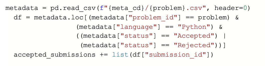
The Project CodeNet Dataset consists of a very large collection of source files, extensive metadata, tooling to access the dataset and make tailored selections, and documentation. It is a large-scale dataset with approximately 14 million code samples, each of which is an intended solution to one of 4000 coding problems. The code samples are written in over 50 programming languages (the dominant languages are C++, C, Python, and Java) and they are annotated with a rich set of information, such as its code size, memory footprint, cpu run time, and status, which indicates acceptance or error types. The data and metadata are organized in a rigorous directory structure. At the top level sits the Project CodeNet directory with several sub-directories, data, metadata, and problem descriptions: data is further subdivided into a directory per problem and within each problem directory, directories for each language. The language directory contains all the source files supposed to be written in that programming or scripting language. Out of the vast dataset we used only python dataset and for the better accuracy of our prediction we used only the accepted codes solution.
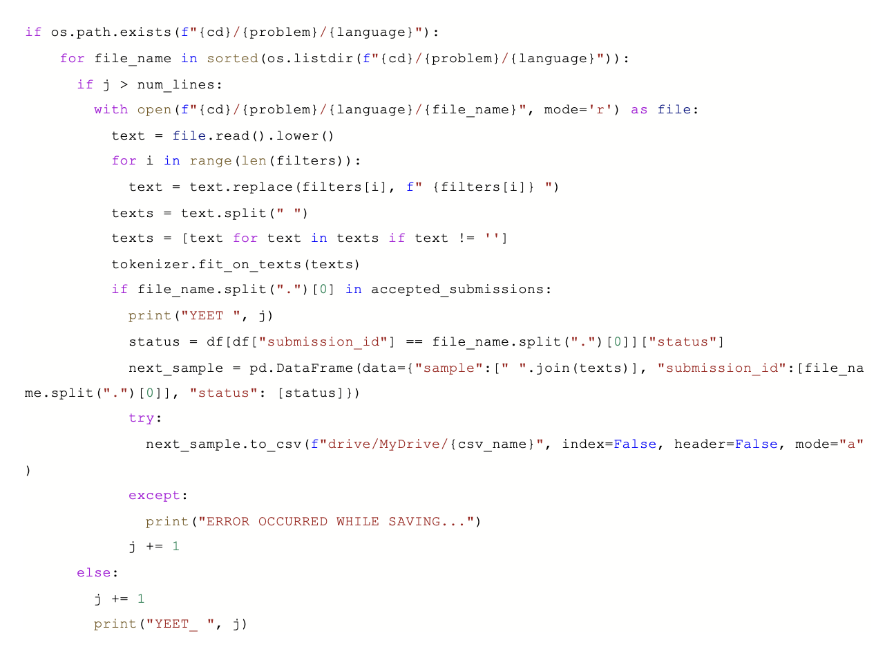
To create a custom dictionary, we must tokenize each element of the code. Tokenization is essentially splitting a phrase, sentence, paragraph, or an entire text document into smaller units, such as individual words or terms. Each of these smaller units are called tokens. Since we are tokenizing code samples and not a text, we must create a filter which can break the code as per our interest.
filters='!"#$%&()*+,-./:;<=>?@[\\]^_`{|}~\t\n1234567890'
We used the above filter string with the python method split() to split it into each dictionary element. What it does is it will take each string item from our filter and create a list and save it to our dictionary.
The output of the above codes will give us a dictionary which contains all the tokenized code samples.
We will use the above tokenized dictionary to train our tokenizer. For the training of the tokenizer we first start with all the characters present in the training corpus as tokens. Identify the most common pair of tokens and merge it into one token. Repeat until the number of tokens has reached the size we want.
2.2 Creating Word Embeddings
2.2.1 Summary of Word2Vec. One of the best known methods for creating meaningful word embeddings is a method called Word2Vec, created by a team of researchers working at Google in 2013.[1]
Word2Vec works by taking as input a text corpus which is used to create a dictionary of one-hot encoded words. For example, if the dictionary contains ten thousand words, and the fiftieth word is “cat”, then the word “cat” will be encoded as a vector of ten thousand zeros, except for a one in the fiftieth position.
The next step in the process is to create a vector that represents the context of the word in a particular sentence. For example, in the sentence “The dog chased the cat” the context words are “dog” and “chased”, and these can both be encoded in the same vector by summing the one-hot encodings of each of these words (using the same process as in the previous step). This new vector will be a context vector for the word “cat”. This process is repeated until all words and all contexts for each word have been converted to vectors.
Finally, a neural network is created that takes as input the word vector and attempts to output the context vector. The dimensionality of the hidden layers of the network are reduced from 10,000 at the input (in this example) to a much smaller dimension (200-300, for example), and then re-expanded to the original dimension to output the context vector.
This architecture forces the network to learn a dense encoding from the sparse inputs. The output of the last small-dimension hidden layer is then used as a vector to represent each word input into the neural network. This learned vector representation contains information about what contexts words appear in, essentially.
2.2.2 Other Word Embedding Methods. Two other well known word embedding techniques are singular value decomposition from a co-occurrence matrix[2], and word embeddings using the Transformer architecture.[3] We currently plan to use the approach from 2.1.1 for any custom word embeddings done for this project, but that may change depending on available time and resources.
2.2.3 Completed Word2Vec Work. So far, we have trained our own word embeddings using several neural network structures in Keras using the methodology described in 2.1.1.
The first neural network architecture we used was an input layer (30,000 dimensional) into a hidden layer (300 dimensional with ReLU activation) into an output layer (30,000 dimensional). Using this architecture, we were able to create a 300 dimensional latent space that effectively predicted the correct word based on context with a 95% accuracy.
The second (more successful) neural network architecture had the same input and output layers, but the hidden layers were 3X hidden layers, each with 30 neurons (ReLU activation). This deeper network allowed us to create arguably better word embeddings, with a smaller dimensional latent space (30, instead of 300), while achieving higher accuracy (97.5%, instead of 95%).
To achieve this high of an accuracy, we trained the model for tens of thousands of epochs - an approach that is probably not advisable for most machine learning models this size because of the possibility of overfitting. In this case, though, the goal of our model was information compression, and our model would never see any “new” data other than what it was trained on, so the inability to generalize is not really a concern.
When we use these custom word embeddings in our RNN, LSTM, and Transformer models, we will compare the results with pre-trained word embedding models like GLoVE.
2.3 N-gram Code Completion
Models that assign probabilities to sentences or sequences of words and can be used to find the most likely continuation of a sequence, are called language models. Among them, is the n-gram language model, which assigns probabilities to sequences out of n words, called the n-grams. A one-word sequence is a unigram, pairs of words are referred to as 2-grams or bigrams, 3-grams or trigrams are sequences of three words, and so on.[7] Examples of bigrams might be "he ate", "ate the", "the whole" and "whole pizza", whereas trigrams would look like "he ate the", "ate the whole", and "the whole pizza".
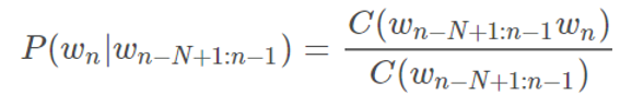
To describe the conditional probability of a word w based on history h, we use the following notation:
P(w | h)
Here is a more concrete example: if we have a sentence "he ate the whole pizza", and want to compute the probability of the word "pizza" given that the previous words are "he ate the whole", we can express it as a conditional probability:
P(pizza|he ate the whole)
To estimate this probability, we can use relative frequency: we need to compute the number of occurrences of "he ate the whole", as well the number of occurrences of the sentence "he ate the whole pizza", and divide the latter by the former:
P(pizza|he ate the whole)
= C(he ate the whole pizza) / C(he ate the whole)
2.3.1 Completed N-gram Work. We created a simple pipeline function which splits the dataset by the <EOS> sample token. This <EOS> token suggests that it is the end of a particular code block. We also remove leading and trailing spaces and tokenize each word of code using nltk.word_tokenize.
We then split our tokenized code samples into training, testing and validation sets. As our dataset is quite big, we only used those words that appear k times in our dataset. For this, we created a function that creates a frequency dictionary.
To enable the model to handle code tokens that are not present in the training corpus, we created a closed_vocabulary containing only those code tokens according to the count_threshold parameter.
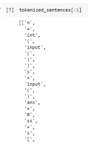
Tokenized Code samples
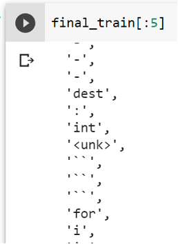
We then add <unk> tokens to those code tokens which are not there in the closed_vocabulary.
Final Training Corpus which contains <unk> tokens.
This function calculates the priority of the next token given our previous n-gram:
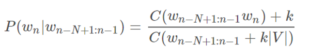
We had to consider what if we came across a n-gram that wasn’t in the training set. Then our denominator in the above function would be zero and our definition for the probability would become invalid. Thus, we use k-smoothing, which adds a positive constant k to each numerator and k×|V| in the denominator, where |V| is the number of words in the vocabulary. This ensures any n-gram with zero count has the same probability of 1 / |V|. Thus, our original estimation gets modified to:
Reference[13]:https://www.kaggle.com/sauravmaheshkar/auto-completion-using-n-gram-models
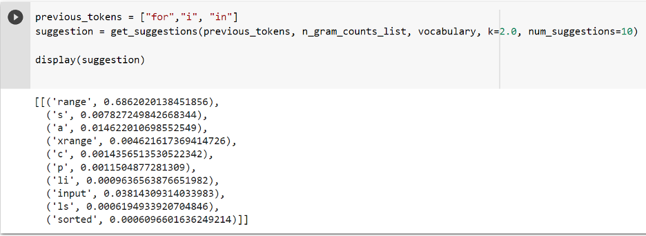
We can see that for the input of “for i in”, the n-gram model outputs the top 10 suggestions with “range” as having the highest probability. This makes sense because when we write a for loop, we usually write it as “for i in range(0, 10)”
2.4 RNN Code Completion
2.4.1 Summary of Recurrent Neural Networks. Recurrent neural networks (also known as RNNs) pass some knowledge about the previous time step into the neural network processing for the current time step. This approach was used to build Pythia, a code completion tool built in to Intellicode (an extension for Visual Studio Code).[4]
2.4.1 Implementation of Recurrent Neural Networks. Before the implementation of recurrent neural networks, we first define the inputs/outputs design for training these networks. Overall, we model the entire dataset as a sequence of tokens and aim to predict the next token. For each token, we consider the last 10 tokens as context because programs should not have a longer context of narrative like spoken languages.
Before creating the table for this design, we generated tokens corresponding to different code text using python interpreter tokenization tools. It is essential that we do so because token s in natural languages can be generated by Tensorflow’s SDK tools based on spaces, but it’s not possible on programming languages because the grammar is different which is understandable to the compiler. The unique set of tokens generated are over ~200000 which includes variable names, operators and comments.
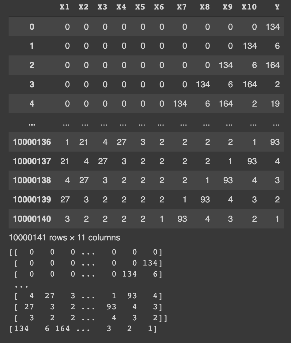
Then we split the entire corpus as a table of X1..X10 inputs and Y as output, where X1 to X10 are 10 previous tokens or an empty string if there was none. This defines the input layer of our neural network based designs as shown in Fig.2.4.1.1.
Next we build a Vanilla RNN containing 256 nodes, with 2 dense feed forward layers of 256 nodes, dropout regularization and Relu activation. The last layer gives Softmax output for us to be able to predict a token from the most commonly used tokens of the corpus vocabulary. This makes it a context aware prediction for code completion rather than simply completing the word or template as in IDE level code completion.
The accuracy we get is ~75% which could be further improved by fine tuning the network.
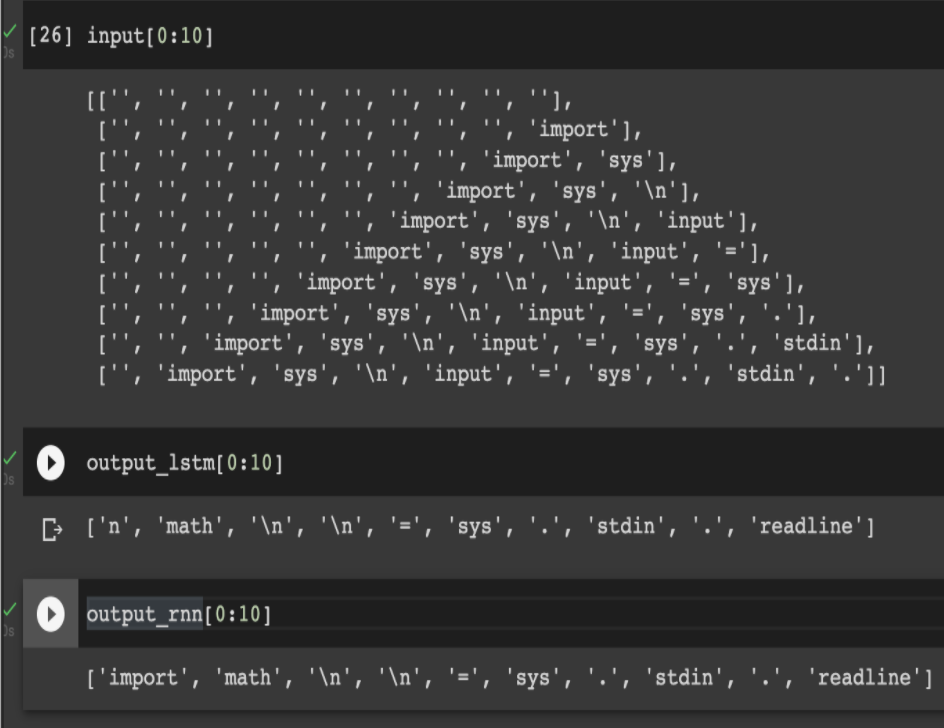
Fig.2.4.1.1 Sample tables created and their translation predictions mapped from tokens to code
2.4.2 Weaknesses of Recurrent Neural Networks. Basic RNNs suffer from the vanishing gradient problem. To rephrase, this means that the network can only remember so far back in time. If an important event occurred in a text series 1000 words ago, the RNN would likely not be able to remember that event long enough to make the connection to the current event. Long Short Term Memory (LSTM) models try to fix this problem.
2.5 LSTM Code Completion
In [9], the team decided to train a machine learning model to sort completions from a code completion library rather than have the model generate the completion itself. They decided on doing this because some code completion libraries complete one keyword at a time ensuring that completions are syntactically correct. In order for them to use the dataset quickly, they created a new ML pipeline which takes a python library and transforms it into a dataset suitable for their model. Their best performing model takes two inputs, 40 latest tokens from the code written so far and a completion from Jedi: an open source static analysis tool written in Python for Python with a focus on code completion.
In order to sort the completions from Jedi, they created a model that performs binary classifications on the completions. Since their model will return scores between 0 and 1, they are able to sort the jedi completions based on the score that their model gives.
Upon evaluation, they found that the JEDI LSTM Sorter model required a person to put in 80% of the keystrokes to achieve a significantly decent code completion. However, the probability of achieving the top 3 completions was 90% which is significantly high in comparison to the traditional JEDI model.
In [10], they define how a standard LSTM works and how traditional RNN suffer from hidden state bottleneck which is where all the information about the current sequence is composed into a fixed sized vector. In order to mitigate this problem, they propose an attention mechanism which is incorporated into the traditional LSTM. They keep an external memory of previous hidden states. At a certain point of time, the model uses an attention layer to compute the relation between the previous states and the hidden states. The model then produces a summary context vector. With the attention of LSTM, they received an accuracy of 80.6% in comparison to Vanilla LSTM with an accuracy of 79% in completion of Python based code.
In [11], they also tried to implement LSTM and RNN where they use a dense layer after the GRU cell to get the scores for each output token. However, they did not achieve good accuracy with the LSTM model.
2.4.1 Implementation of LSTM Networks.
The implementation of LSTM is similar to that of RNN. For building the model architecture, we used the same set of hyper parameters as we did for RNN. We also attempted to predict as a classification problem over the entire corpus tokens set instead of selecting the most frequently occurring elements as is the practice in text completion when dealing with natural languages. This is because of the sparse distribution of the tokens. For completing phrases such as variable names, we can no longer rely on the most commonly spoken textual tokens, rather we need to be aware of the context and pick up the most recently used variable/method name as the case may be. We want our network to be aware of such context. This brings in challenges of training the network, because of the size of the data and computation resources that are expensive on larger models and data sizes.
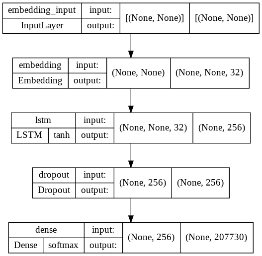
With the above hypothesis, we build the LSTM network with inputs first passing tokens to a trainable embedding unlike a pre-trained word embedding layer of 32 dimension. This further forwards to an LSTM layer containing 256 nodes. And finally, we add 2 dense feed forward layers of 256 nodes each, dropout regularization and Relu activation is used just as in Vanilla RNN. The last layer gives Softmax output for us to be able to predict a token from the entire token corpus which is approximately ~200000 .
We trained on 20 epochs and got 84.1% accuracy which is great performance on a set of this size. While this performance is great on its own, there could be further variations to beat this. However, Each epoch took around 3-4 hours and due to resource constraints, we could not experiment with more sets of hyperparameters and acknowledge it as a part of our future work.
2.6 Transformer Code Completion
2.6.1 Summary of Transformer Networks. Transformers were introduced in 2017 by Google Brain in [12] and have been, in direct or indirect way, the preferred model for NLP applications, replacing the more traditional RNN and its variants such as LSTM or GRUs. As an only attention based model, without RNN layers the transformers are capable of having extremely long term memory. They overcome sequential dependency of RNNs and also tackle its vanishing gradient difficulty. They allow for processing phrases in any order and provide meaning by focusing on context around it. This ability allows training to be parallelizable and we can process much larger datasets that were hard to do before. A direct consequence of this ability has led to evolution of pre-trained models like BERT ((Bidirectional Encoder Representations from Transformers) and GPT (Generative Pre-trained Transformer) on wikipedia corpus which are used in production by Google search.
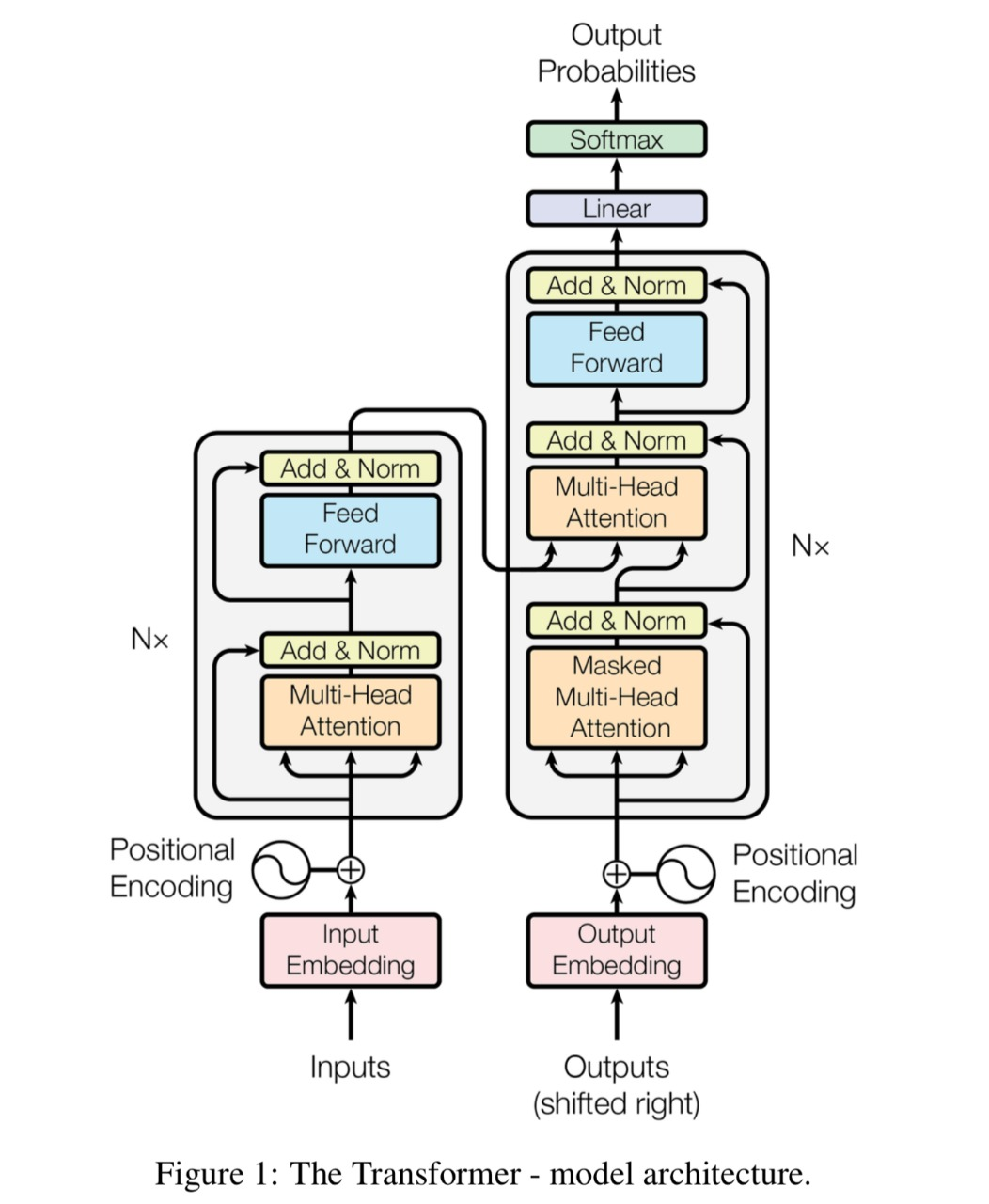
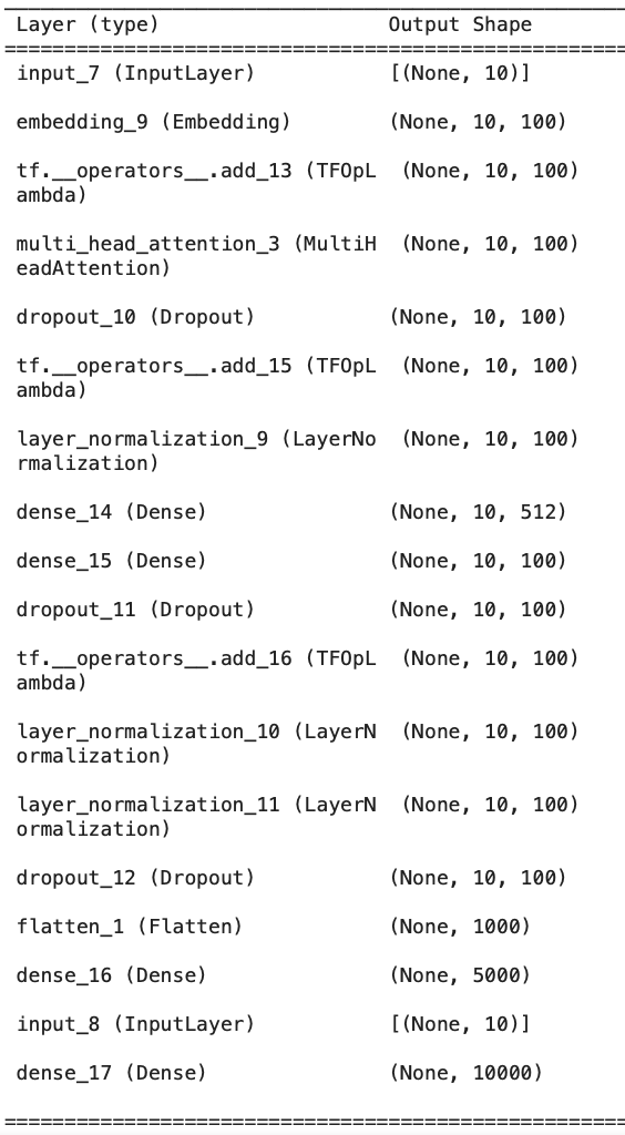
The transformers consist of several layers and are expensive to build on large sentences. The layers are grouped into 2 categories: encoder and decoder. The encoder takes in word embeddings from input text and adds positional encodings. Then a multi-head attention layer computes attention weights which are then passed to feed forward layers. The output of this encoder is then passed to decoder which combines the encoder’s output to target text’s word embeddings and positional encodings. Below is the architecture proposed by authors in [12].
2.6.2 Completed Transformers Work. We’ve attempted to train both a complete transformer model (following the above figure), and just the decoder section (see the left side of the above figure). The transformer model was attempting to predict which token (out of the 10,000 most common tokens) was most likely to occur next. We have not yet decided if limiting the possible outputs to the top 10,000 most frequent tokens was a good idea or not. When training our RNN and LSTM models, we did not limit the dictionary size to 10,000. Both models reported a ~75% training accuracy and a ~90% training top-5 accuracy. When testing the models, though, both seemed extremely biased towards predicting newline characters as the next token. This makes sense, given that the newline character is one of the most frequent tokens used during coding in Python.
While we did not have time to fix this issue, we did begin working on a few ideas for solutions. The most obvious solution idea is to weight each token in the loss function so that incorrectly classifying a newline character has less negative impact than incorrectly classifying an “if-then” statement. The most straightforward method for reweighting classes is to reweight classes based on frequency so that the least common classes contribute the most to the loss when misclassified, while common token classes (like the newline character) contribute very little to the loss when misclassified. The problem with this approach is that we don’t want to severely punish our model for missing some obscure token, but reweighting the model in this way would do exactly that.
We also worked with the idea of just dropping the first two most popular tokens (newline and unknown tokens) from our predictions completely, given that both of these predictions provide minimal value to the programmer while also severely skewing our class balance. This idea was worked with briefly, but we were not able to pursue it further due to time constraints.
See the following image for the Transformer encoder (left half) architecture:
2.6.3 Lessons Learned from Transformers. While our transformer models were not particularly successful on testing data, we did learn a lot about transformer networks during our project. Two key parts of what makes transformer networks successful are the use of self attention layers and positional embeddings to preserve sequence.
To sum up, self attention layers compare each item (in this case, word) in a sequence to every other item in that sequence. This allows the model to learn how important every other word is in predicting the word it is currently focusing on. Positional embeddings are added to the token embeddings so that the order of the sequence can be understood by the attention layer. Without this summation, the model is order-agnostic, which would obviously not be good for a text generation or code completion model.
For more helpful information about Transformer networks, we highly recommend reading “Attention is All You Need” [12].
3 Conclusion
Next we present some of the major results and observations from comparing the different experiments.
3.1 Project Description
3.1.1 Project Summary. We worked to replicate each section of the related work, some sections being more successful than others. We used an n-gram code completion model as the baseline to compare all other techniques to. The goal is to find the next word in a sequence, given the preceding text. The specific programming language we’re focusing on is Python, though these same techniques should apply seamlessly to other languages.
3.1.2 Proposed Dataset. The dataset we used is the IBM CodeNet dataset[5] which includes millions of code samples from C++, Python, and several other less common languages. These additional languages could come in useful for creating models that
3.2 Goal Conclusions
3.2.1 First Goal. The goal of the project has been two-fold. First and primarily, we wanted to recreate past successful code completion methods. This goal has been achieved with n-gram, RNN, and LSTM code completion methods. Transformer networks require additional work before we can consider that goal met for that type of network.
3.2.1 Second Goal. Second, we wanted to be able to clearly explain each method used. We believe this second goal has been a success for everyone involved in the project.
4 Model Evaluation
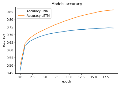
We withheld a portion of the CodeNet python dataset to use as a validation and testing dataset. The evaluation metric used was accuracy, like used in previous code completion projects.[4] Our LSTM model achieved an accuracy of 86.23% on a validation dataset, beating our RNN model by 11.5%. On the 20th epoch, when training ended for our LSTM model the accuracy was still increasing, as can be seen in the following plot:
This trend strongly indicates that there is future room for improvement in both of these models, but particularly with the LSTM model.
Given the issues with the transformer models, we do not have a final model accuracy worth sharing. That part of the project is far too incomplete, and requires a good deal of further work before good results can be expected.
5 Future Work
There are several big things that would make good additions to this project that we’re aware of.
1) Increasing the breadth of our Python dataset is a good first step. The IBM dataset is composed of code meant to solve a fairly limited set of problems. Expanding this dataset to include a larger set of solved problems would be a good starting point.
2) A good second step to work on would be improving the transformer networks and working on solving the class imbalance problem. Given that transformer networks are state of the art for sequence generation models, we believe that the issues we’re having with them are not due to the model structure, but are rather due to our use of the models and our data preprocessing.
3) Further work with model architecture tuning and hyperparameter tuning could help improve our working models even further. Striking a balance between model size, model accuracy, and avoiding overfitting is a surprisingly difficult task. This step is potentially very resource intensive.
4) Pre-formatting the code we’re training on to PEP-8 could help with data preprocessing by removing inconsistencies in our dataset.
5) We would like to expand our work to other common programming languages (Java, C++, Go, JavaScript, etc.). Once data preprocessing is complete for each language, this process should be fairly straightforward, as it will be primarily focused on waiting for the same model architectures to train on different datasets.
6) Another interesting possible use-case for Transformer networks is for translating code from one coding language to another (i.e. Java to Python). Given that Transformers are frequently used for language translation, this use-case seems entirely plausible.
7) Finally, we would like to deploy our code completion models as add-ons for integrated development environments after we’ve ironed out the small set of issues that we’re having.
REFERENCES
[1] Mikolov, Tomas, et al. "Efficient estimation of word representations in vector space." arXiv preprint arXiv:1301.3781 (2013).
[2] Pennington, Jeffrey, Richard Socher, and Christopher D. Manning. "Glove: Global vectors for word representation." Proceedings of the 2014 conference on empirical methods in natural language processing (EMNLP). 2014.
[3] Laskar, Md Tahmid Rahman, Xiangji Huang, and Enamul Hoque. "Contextualized embeddings based transformer encoder for sentence similarity modeling in answer selection task." Proceedings of The 12th Language Resources and Evaluation Conference. 2020.
[4] Svyatkovskiy, Alexey, et al. "Pythia: AI-assisted code completion system." Proceedings of the 25th ACM SIGKDD International Conference on Knowledge Discovery & Data Mining. 2019.
[5] "Project CodeNet - IBM Developer." 5 May. 2021, https://developer.ibm.com/exchanges/data/all/project-codenet/. Accessed 13 Feb. 2022.
[6] Hindle, Abram, et al. “On the Naturalness of Software.” Communications of the ACM, vol. 59, no. 5, 2016, pp. 122–131., doi:10.1145/2902362.
[7] Jurafsky, Daniel, and James H. Martin. “Speech and Language Processing (3rd Ed. Draft) Dan Jurafsky and James H. Martin.” Speech and Language Processing, web.stanford.edu/~jurafsky/slp3/.
[8] Yang, Yixiao, and Chen Xiang. “Improve Language Modelling for Code Completion through Learning General Token Repetition of Source Code.” International Conferences on Software Engineering and Knowledge Engineering, 2019, doi:10.18293/seke2019-056.
[9] Barath, Boris. “ML Code Completion.” Imperial.ac.uk, www.imperial.ac.uk/media/imperial-college/faculty-of-engineering/computing/public/1920-ug-projects/distinguished-projects/ML-Code-Completion.pdf.
[10] Li, Jian, et al. “Code Completion with Neural Attention and Pointer ... - IJCAI.” Ijcai.org, 2018, www.ijcai.org/Proceedings/2018/0578.pdf.
[11] Das, Subhasis, and Chinmayee Shah. “Contextual Code Completion Using Machine Learning.” Stanford.edu, web.stanford.edu/~chshah/files/contextual-code-completion.pdf.
[12] Ashish Vaswani, et. al, “Attention is all you need”, 31st Conference on Neural Information Processing Systems (NIPS 2017).
[13] Sauravmaheshkar. (2021, March 6). Auto-completion using N-Gram models. Kaggle. Retrieved April 28, 2022, from https://www.kaggle.com/sauravmaheshkar/auto-completion-using-n-gram-models